Style Transfer in Heraklion
Christos Hadjinikolis, 15 August 2020
I am currently in Crete for my annual get away. Crete is an amazing island with many beautiful places to visit and a vast history that goes all the way back to the Minoans in 3500 BC.
 One of the things I love doing whenever I am here is strolling around the city of Heraklion and taking pictures of the many hidden alleys,
which reveal an amazing graffiti culture! I really wanted to write about it in my blog and I thought that maybe I can do so
by using some amazing images I gathered just last week in a style-transfer post. So this is it: “Style Transfer in Heraklion”.
A bit of history: A Neural Algorithm of Artistic Style
Neural Style Transfer (NST) is a class of algorithms that process images to adopt the visual style of another image. A seminal paper that introduced this concept was “A Neural Algorithm of Artistic Style” by Leon A. Gatys, Alexander S. Ecker and Matthias Bethge. In their work, the authors emphasize that:
“…representations of content and style in Neural Networks are seperable”.
This is the foundation of this work, since if these two notions are indeed separable then provided two images you can get the style of the first, the content of the second and merge them together. So, how is this done exactly?
Delving into the details

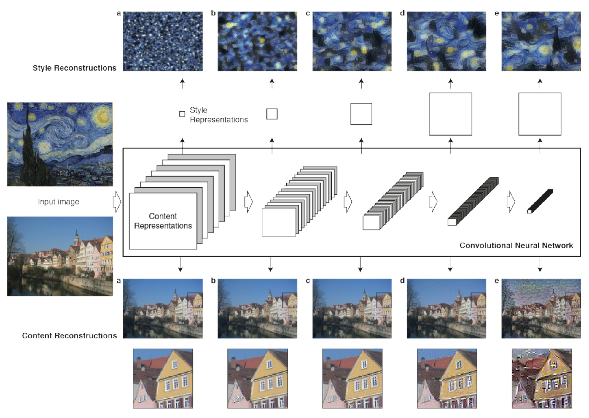
The first figure in the paper shows the original setup and how a pre-trained NN, referred to as VGG19, was modified to do NST. What is VGG19?
Well, the basic building blocks of traditional convolutional networks are the following layers:
- a convolutional layer (with padding to maintain the resolution);
- a non-linear activation layer such as a ReLU, and;
- a pooling layer such as a max pooling layer.
A VGG block consists of a sequence of convolutional layers, followed by a max pooling layer for spatial down-sampling.
What we are interested in is how this network will respond to the inputs.
Retrieving the content
Notice that the authors prefer to use paintings for the style and a random image; it seems like these combinations work best. The main idea is abstracting the content and putting more emphasis on the style!
At the top left you see “The Starry Night” by Vincent van Gogh and below it is just a random content image; let’s start with the latter.

Provided both an input (style) image and a content image, each neuron and respectively each layer in the NN will either activate or it won’t. Each image is processed, or better yet filtered, in a different way (by nature of the activation or not of different neurons). Looking at how the content image is gradually filtered in the above image you will notice that the first layer leaves the image seemingly intact. But looking all the way to the last filtered output you see that this is not the case at all; shapes are there but the inside is not so much the same. This is because of how the resulting high-level features are generated on earlier abstractions of the same image produced by previous layers. This is the intended behaviour to retrieve the content.
Retrieving the style

So, for the style, the authors explain that they have built a new feature-space, which focuses on the style of an input image on top of the original CNN representations. The style representation computes correlations between the different features in different layers of the CNN. They reconstruct the style of the input image from style representations built on different subsets of CNN layers and this results in images that match the style of the input on an increasing scale while discarding information of the arrangement of the scene.
It’s all in the formulas (or formul$ae$)
The authors also discuss the impact of the number of layers used to infer the style or the content of images before they are merged
(visually depicted in Figure 3 of the paper).  In the first row (A) only one layer is used in contrast to 5 layers used at the bottom row where the result is much better.
To generate the images which are a mixture of the content of an image-A with the style of another (image-B) the authors explain that they jointly minimise the distance of a “white noise” image from the content representation of image-A in one layer of the network and the style representation of image-B in a number of layers of the CNN. This is gracefully captured by the below loss function:

where $\overrightarrow{p}$ is image-A (usually a photograph where we care about the content) and $\overrightarrow{a}$ is image-B (usually a painting where we care to retrieve the style). Then $\alpha$ and $\beta$ respectively concern weighting factors for content and style reconstruction.
Going back to Figure 3 of the paper, looking at it from left to right we see what happens when we tweak these weighting factors ($\alpha$ and $\beta$). The left-most column concerns cases where $\alpha$ is low compared to $\beta$ and the right-most layer is the other way around. These two factors are practically the optimisers of the content and style errors respectively. If $\alpha$ is high, it means that content error is more important and vice-versa for increasing $\beta$.
The objective of the formula is to minimize $\mathcal{L}_{total}$. $\overrightarrow{x}$ is the image that we are gradually building through multiple iterations and it initially comes either from the photograph ($\overrightarrow{p}$) or it is initialised as white noise. $\alpha$ and $\beta$ are the weights that we need to set, and they are basically our hyper-parameters in this problem.
What is now left is understanding \(\mathcal{L}_{content}\) and \(\mathcal{L}_{style}\).
$\mathcal{L}_{content}$
Here is where everything gets a bit complicated but at the same time, you get to piece everything together nicely.
$\mathcal{L}_{content}$ is described as the squared-error loss between two feature representations: one concerned with the random photograph
$\overrightarrow{p}$ and the generated image $\overrightarrow{x}$ which is originally a white noise image.
 $P^l$ and $F^l$ are the respective feature representations for the two images in layer $l$. The authors used the feature space provided by the 16 convolutional and 5 pooling layers of the 19 layer
 VGG Network.
Here, $F^l$ represents an activation function ($F$) at a given layer $l$ or, plainly, a bank of non-linear filters for that layer. The complexity of these filters increases
with the position of the layer in the network. $F$ is practically a matrix of size $N\times M$ where $N$ is the number of filters within
a given layer with $N_l$ feature maps of size $M_l$; the latter is the height $\times$ width if the feature map.
So, a given input image $\overrightarrow{x}$ is encoded in each layer of the CNN by the filter responses to that image.
To visualise the image information that is encoded at different layers of the hierarchy the authors perform gradient descent
on the white noise image to find another image that matches the feature responses of the original image.
 So, the approach is to gradually changes the initially random image $\overrightarrow{x}$ until it generates the same response in a certain layer of the CNN as the original image.
$\mathcal{L}_{style}$
The style loss function is described by the following equation:

which is basically a sum of the weighted distances between feature correlations across the different filter (layer) responses for two images:
- the original image $\overrightarrow{a}$, and;
- a white noise image $\overrightarrow{x}$, used to generate a style representation of the original image.
Let’s break this down a bit more; what are these feature correlations? Practically they are a way to express a relationship between a feature map $F$ and
the filters ($i$ and $j$) of the different layers ($l$) applied on it. This is beautifully expressed as a matrix of all possible inner
products between the generated set of feature vectors, called a “Gram matrix $G$”, as per the below equation:

One such matrix is generated for each of the two images (the original $\overrightarrow{a}$ and $\overrightarrow{x}$), namely $A_{ij}^l$ and $G_{ij}^l$, and a squared distance is calculated between these two. The objective is to minimise the distance. So, practically, as with every ML problem, what we have is an optimisation problem and a cost function! Minimising this distance can be achieved through the application of gradient descent using standard error back-propagation to adjust the weight values of equation $5$.
Putting it all together
Finally, in order to generate the final image with the style transfer, we return to equation 7, which practically jointly minimises the distance of a white noise image from the content representation of the photograph in one layer of the network and the style representation of the painting in a number of layers of the CNN. The authors also note that:
For image synthesis they found that replacing the max-pooling operation by average pooling improves the gradient flow and one obtains slightly more appealing results.
That’s it! So, what’s left now is getting our hands dirty!
Using PyTorch for Style transfer
If you following this link to the official
PyTorch website you will find a very well written tutorial on how to apply style transfer with PyTorch. I provide
my own take of it $\rightarrow$here$\leftarrow$. You
can follow the link to the python notebook and copy-paste the code to give it a try.

I intend to work on creating a package for it and will provide an updated post on it once I do (it will be developed in the same repo as the link). The intention is to be able to style images through the packages through an intuitive api that would take the image to be styled as the input and a choice between famous images that will be available through the package (provided as a text parameter) to produce the desired output (along with some other flags and side parameters). Something like:
import pytorch_style_transfer as pst

pst.generate(
    input_image_path="path_to_input_image",
    style="starry_night",
    resolution=128,
    output_dir="path/to/output")
Enjoy some of the outputs:
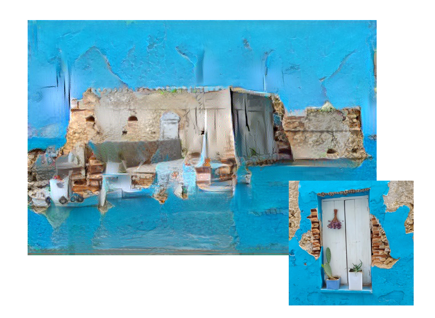
Here are some of the results of this work. I tried blending the fortress of Koules with 4 different grafittis I was able to photograph.
The original picture:

The result is not always great, but it was still very interesting to try:


That’s it!
Remember to like my post and re-share it (if you really liked it)!
See you soon!
![]() Register to the ML-Affairs RSS Feed
Register to the ML-Affairs RSS Feed
Just had a go at style-transfer #cnn #deep_learmning. Have a look at my latest blog-posthttps://t.co/oTEdZIL1T0
— Christos Hadjinikoli (@chatzinikolis) August 16, 2020
